If you run an e-commerce website a classical problem is to rank your product offering in the search page in a way that maximises the probability of your items being sold. For example if you are selling shoes you would like the first pair of shoes in the search result page to be the one that is most likely to be bought.

Thanks to the widespread adoption of machine learning it is now easier than ever to build and deploy models that automatically learn what your users like and rank your product catalog accordingly. In this blog post I'll share how to build such models using a simple end-to-end example using the movielens open dataset.

Introduction

Imagine you have an e-commerce website and that you are designing the algorithm to rank your products in your search page. What will be the first item that you display? The one with the best reviews? The one with the lowest price? Or a combination of both? The problem gets complicated pretty quickly.

A simple solution is to use your intuition, collect the feedback from your customers or get the metrics from your website and handcraft the perfect formula that works for you. Not very scientific isn't it? A more complex approach involves building many ranking formulas and use A/B testing to select the one with the best performance.

Here we will instead use the data from our customers to automatically learn their preference function such that the ranking of our search page is the one that maximise the likelihood of scoring a conversion (i.e. the customer buys your item). Specifically we will learn how to rank movies from the movielens open dataset based on artificially generated user data. The full steps are available on Github in a Jupyter notebook format.

Prepare the training data

To learn our ranking model we need some training data first. So let's generate some examples that mimics the behaviour of users on our website:

The list can be interpreted as follows: customer_1 saw movie_1 and movie_2 but decided to not buy. Then saw movie_3 and decided to buy the movie. Similarly customer_2 saw movie_2 but decided to not buy. Then saw movie_3 and decided to buy.

In a real-world setting scenario you can get these events from you analytics tool of choice, but for this blog post I will generate them artificially. To do that we will associate a buy_probability attribute to each movie and we will generate user events accordingly.

Our raw movies data looks like this:

and this is an example of a movie from the dataset:

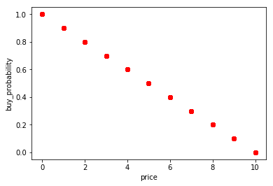
Let's assume that our users will make their purchase decision only based on price and see if our machine learning model is able to learn such function. For this dataset the movies price will range between 0 and 10 (check github to see how the price has been assigned), so I decided to artificially define the buy probability as follows:

With that buying probability function our perfect ranking should look like this:

No rocket science, the movie with the lowest price has the highest probability to be bought and hence should be ranked first. Now let's generate some user events based on this data. Each user will have a number of positive and negative events associated to them. A positive event is one where the user bought a movie. A negative event is one where the user saw the movie but decided to not buy.

Before moving ahead we want all the features to be normalised to help our learning algorithms. So let's get this out of the way. Also notice that we will remove the buy_probability attribute such that we don't use it for the learning phase (in machine learning terms that would be equivalent to cheating!).

finally using the EventsGenerator class shown below we can generate our user events. For simplicity let's assume we have 1000 users and that each user will open 20 movies. Real world data will obviously be different but the same principles applies.

and this is how everything gets glued up together. The EventsGenerator takes the normalised movie data and uses the buy probability to generate user events.

And this is how one of these events look like:

In this case we have a negative outcome (value 0) and the features have been normalised and centred in zero as a result of what we did in the function build_learning_data_from(movie_data).

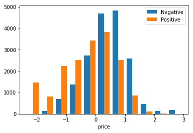
If we plot the events we can see the distribution reflect the idea that people mostly buy cheap movies. Again price is centred in zero because of normalisation.

Train our models

Now that we have our events let's see how good are our models at learning the (simple) buy_probability function. We will split our data into a training and testing set to measure the model performance (but make sure you know how cross validation works) and use this generic function to print the performance of different models.

training the various models using scikit-learn is now just a matter of gluing things together. Let's start with Logistic Regression:

which gives us the following performance

We can do the same using a neural network and a decision tree. This is a neural network with 23 inputs (same as the number of movie features) and 46 neurons in the hidden layer (it is a common rule of thumb to double the hidden layer neurons).

and this is the performance we got

and finally with decision trees

which gives us the following performance

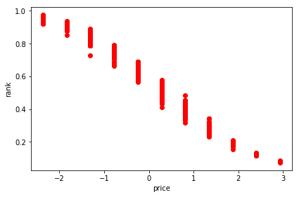
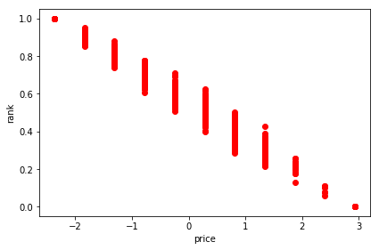
We can plot the various rankings next to each other to compare them. The shape of the ranking curve is very similar to the one we used to define the buy_probability which confirms that our algorithms learnt the preference function correctly.

The shape isn't exactly the same describing the buy_probability because the user events were generated probabilistically (binomial distribution with mean equal to the buy_probability) so the model can only approximate the underlying truth based on the generated events.

What's next

Once you got your ranking estimates you can simply save them in your database of choice and start serving your pages. With time the behaviour of your users may change like the products in your catalog so make sure you have some process to update your ranking numbers weekly if not daily. It could also be a good idea to A/B test your new model against a simple hand-crafted linear formula such that you can validate yourself if machine learning is indeed helping you gather more conversions.

If you prefer to wear the scientist hat you can also run the Jupyter notebook on Github with a different formula for buy_probability and see how well the models are able to pick up the underlying truth. I did tried a linear combination of non-linear functions of price and ratings and it worked equally well with similar accuracy levels.

Finally, a different approach to the one outlined here is to use pair of events in order to learn the ranking function. The idea is that you feed the learning algorithms with pair of events like these:

With such example you could guess that a good ranking would be movie_3, movie_2, movie_1 since the choices of the various customers enforce a total ordering for our set of movies. Despite predicting the pairwise outcomes has a similar accuracy to the examples shown above, come up with a global ordering for our set of movies turn out to be hard (NP complete hard, as shown in this paper from AT&T labs) and we will have to resort to a greedy algorithm for the ranking which affects the quality of the final outcome. A more in-depth description of this approach is available in this blog post from Julien Letessier.

Conclusion

In this blog post I presented how to exploit user events data to teach a machine learning algorithm how to best rank your product catalog to maximise the likelihood of your items being bought. We saw how both logistic regression, neural networks and decision trees achieve similar performance and how to deploy your model to production.

Looking forward to hear your thoughts in the comments and if you enjoyed this blog you can also follow me on twitter.

---

Also published on Medium.